Handling large data with R and Python

Etienne Bacher

2026-01-16

Plan for today

1. Motivation

2. Introduction to lazy evaluation

3. How to use Polars

4. More advanced concepts

5. Alternative tools

1. Motivation

Motivation

The use of big data in all disciplines is growing:

• full censuses
• genomics data
• mobile phone data
• and more…

Motivation

Usually, we load datasets directly in R (or Stata, or Python, or something else).

This means that we are limited by the amount of RAM¹ on our computer.

We might think that we need a bigger computer to handle more data.

1. Random Access Memory, where the data can be accessed by the programs.

Motivation

But we can’t necessarily have a bigger computer.

And we don’t necessarily need a bigger computer in the first place.

Multiple tools exist for user-friendly large data handling:

• polars
• arrow
• DuckDB
• etc.

Motivation

But we can’t necessarily have a bigger computer.

And we don’t necessarily need a bigger computer in the first place.

Multiple tools exist for user-friendly large data handling:

• polars
• arrow
• DuckDB
• etc.

Polars

polars is a recent DataFrame library that is available in several languages:

• Python
• R
• Rust
• and more

Very consistent and readable syntax.

Built to be very fast and memory-efficient thanks to several mechanisms.

Polars

The main mechanism is called lazy evaluation.

The next section is language agnostic: it is based on concepts, not language features.

2. Introduction to lazy evaluation

Eager vs Lazy

Eager evaluation: all operations are run line by line, in order, and directly applied to the data. This is the way we’re used to.

### Eager

# Get the data...
my_data = eager_data
  # ... and then sort by iso...
  .sort(pl.col("iso"))
  # ... and then keep only Japan...
  .filter(pl.col("country") == "Japan")
  # ... and then compute GDP per cap.
  .with_columns(gdp_per_cap = pl.col("gdp") / pl.col("pop"))

# => get the output

Eager vs Lazy

Lazy evaluation: operations are only run when we call a specific function at the end of the chain, usually called collect().

### Lazy

# Get the data...
my_data = lazy_data
  # ... and then sort by iso...
  .sort(pl.col("iso"))
  # ... and then keep only Japan...
  .filter(pl.col("country") == "Japan")
  # ... and then compute GDP per cap.
  .with_columns(gdp_per_cap = pl.col("gdp") / pl.col("pop"))

# => you don't get results yet!

my_data.collect() # this is how to get results

Eager vs Lazy

Polars has both eager and lazy evaluation.

When dealing with large data, it is better to use lazy evaluation:

1. Optimize the code
2. Catch errors before computations

1. Optimize the code

The code below takes some data, sorts it by a variable, and then filters it based on a condition:

data
  .sort(pl.col("country"))
  .filter(pl.col("year").is_in([1950, 1960, 1970, 1980, 1990]))

Do you see what could be improved here?

1. Optimize the code

The problem is the order of operations: sorting data is much slower than filtering it.

Let’s test with a dataset of 50M observations and 10 columns:

data
  .sort(pl.col("country"))
  .filter(pl.col("year").is_in([1950, 1960, 1970, 1980, 1990]))

   user  system elapsed 
  5.654   1.986   7.641 

data
  .filter(pl.col("year").is_in([1950, 1960, 1970, 1980, 1990]))
  .sort(pl.col("country"))

   user  system elapsed 
  0.925   0.389   1.314 

1. Optimize the code

There is probably a lot of suboptimal code in our scripts.

Most of the time, it’s fine.

But when it starts to matter, we don’t want to spend time thinking about the best order of operations.

  Let polars do this automatically by using lazy evaluation.

1. Optimize the code

collect()

-> check the code

-> optimize the code

-> execute the code

Examples of optimizations (see the entire list):

• run the filters as early as possible (predicate pushdown);
• do not load variables (columns) that are never used (projection pushdown);
• cache and reuse computations
• and many more things

2. Catch errors before computations

Calling collect() doesn’t start computations right away.

First, polars checks the code to ensure there are no schema errors, i.e. check that we don’t do “forbidden” operations.

For example, pl.col("gdp") > "France" would return the following error before executing the code :

polars.exceptions.ComputeError: cannot compare string with numeric data

A note on file formats

We’re used to a few file formats: CSV, Excel, .dta. Polars can read most of them (.dta needs an extension).

When possible, use the Parquet format (.parquet).

Pros:

• large file compression
• no type inference (as in CSV for example)
• stores statistics on the columns (e.g. useful for filters)

Cons:

• might be harder to share with others (e.g. Stata doesn’t have an easy way to read/write Parquet)

3. How to use Polars

How to use Polars

Polars can be used in Python and in R:

• Python library polars. This is developed directly by the creators of Polars.

• R packages polars and tidypolars.

  • polars is an almost 1-to-1 copy of the Python polars’ syntax
  • tidypolars is a package that implements the tidyverse syntax but uses polars in the background.
  • Those packages are not on CRAN.
  • Both are maintained by volunteers (including myself).

How to use Polars

Workflow:

1. scan the data to get it in lazy mode.

• Python
• R (polars)
• R (tidypolars)

import polars as pl

raw_data = pl.scan_parquet("path/to/file.parquet")

# Or
pl.scan_csv("path/to/file.csv")
pl.scan_json("path/to/file.json")
...

library(polars)

raw_data <- pl$scan_parquet("path/to/file.parquet")

# Or
pl$scan_csv("path/to/file.csv")
pl$scan_ndjson("path/to/file.json")
...

library(tidypolars)

raw_data <- scan_parquet_polars("path/to/file.parquet")

# Or
scan_csv_polars("path/to/file.csv")
scan_ndjson_polars("path/to/file.json")
...

This only returns the schema of the data: the column names and their types (character, integers, …).

How to use Polars

Workflow:

2. Write the code that you want to run on the data: filter, sort, create new variables, etc.

• Python
• R (polars)
• R (tidypolars)

my_data = raw_data
   .sort("iso")
   .filter(
      pl.col("gdp") > 123,
      pl.col("country").is_in(["United Kingdom", "Japan", "Vietnam"])
   )
   .with_columns(gdp_per_cap = pl.col("gdp") / pl.col("population"))

my_data = raw_data$
   sort("iso")$
   filter(
      pl$col("gdp") > 123,
      pl$col("country")$is_in(list(c("United Kingdom", "Japan", "Vietnam")))
   )$
   with_columns(gdp_per_cap = pl$col("gdp") / pl$col("population"))

my_data = raw_data |>
   arrange(iso) |>
   filter(
      gdp > 123,
      country %in% c("United Kingdom", "Japan", "Vietnam")
   ) |>
   mutate(gdp_per_cap =  gdp / population)

How to use Polars

Workflow:

3. Call collect() at the end of the code to execute it.

• Python
• R (polars)
• R (tidypolars)

my_data.collect()

my_data$collect()

my_data |> collect()

How to use Polars

Problem: you don’t know what the data looks like.

Solution: Use eager evaluation to explore a sample, build the data processing scripts, etc. but do it like this:

my_data = (
  pl.scan_parquet("my_parquet_file.parquet")
  .head(100)
  .collect()
)

# then use eager evaluation

Use lazy evaluation to perform the data processing on the entire data.

Polars expressions

To modify variables, we chain Polars expressions:

• Python
• R (polars)
• R (tidypolars)

my_data.with_columns(
  # Compute the average GDP
  pl.col("gdp").mean(),
  # Convert "NEW_YORK" to "New York"
  pl.col("state_name").str.replace_all("_", " ").str.to_titlecase(),
  # Extract the year from a specific date
  year = pl.col("date").dt.year()
)

my_data$with_columns(
  # Compute the average GDP
  pl$col("gdp")$mean(),
  # Convert "NEW_YORK" to "New York"
  pl$col("state_name")$str$replace_all("_", " ")$str$to_titlecase(),
  # Extract the year from a specific date
  year = pl$col("date")$dt$year()
)

library(lubridate); library(stringr)

my_data |>
  mutate(
    # Compute the average GDP
    gdp = mean(gdp),
    # Convert "NEW_YORK" to "New York"
    state_name = state_name |>
      str_replace_all("_", " ") |>
      str_to_title(),
    # Extract the year from a specific date
    year = year(date)
  )

4. More advanced concepts

4. More advanced concepts

• Custom functions

• Streaming mode

• Larger-than-memory output

• Plugins & the rest

Custom functions

Maybe you need to use a function that doesn’t exist as-is in Polars or in a plugin.

You have mainly three options:

1. write the function using Polars syntax

2. collect the data, convert it (to pandas in Python or to a data.frame in R), and use the function you need

3. use a map_ function (e.g. map_elements() or .map_batches()), but this is slower (available only in Python).

Custom functions

Example: let’s write a custom function for standardizing numeric variables.

• Python
• R (polars)
• R (tidypolars)

# Create a custom function to standardize numeric variables
def standardize(x: pl.Expr) -> pl.Expr:
    # The "return" keywords has to be specified (contrarily to R)
    return ((x - x.mean()) / x.std())

(
  my_data
  .with_columns(
    standardize(pl.col("height"))
  )
)

standardize <- function(x) {
  ((x - x$mean()) / x$std())
}

my_data$
  with_columns(
    standardize(pl$col("height"))
  )

standardize <- function(x) {
  ((x - x$mean()) / x$std())
}

my_data |>
  mutate(
    height = standardize(height)
  )

Streaming mode

Streaming is a way to run the code on data by batches to avoid using all memory at the same time.

This is both more memory-efficient and faster.

Using this is extremely simple: instead of calling collect(), we call collect(engine = "streaming").

Tip

The streaming engine will become the default in a few months so you will be able to simply call collect() without the engine argument.

Larger-than-memory output

Sometimes, data is just too big for our computer, even after all optimizations.

In this case, collecting the data will crash the Python or R session. Polars is not a panacea.

What are possible strategies for this?

Larger-than-memory output

1. Reconsider whether you actually need all the data in the session

Maybe you can use aggregate values instead (e.g. district-level statistics instead of individual statistics).

Maybe you just want to export the data to another file: use sink_*() (e.g. sink_parquet()) instead of collect() + write_*().

Larger-than-memory data

2. Eventually… just get a bigger machine

Plugins

Python only (for now)

Polars accepts extensions taking the form of new expressions namespaces.

Just like we have .str.split() for instance, we could have .dist.jarowinkler().

List of Polars plugins (not made by the Polars developers): https://github.com/ddotta/awesome-polars#polars-plugins

GIS and Polars

While there is demand for a geopolars that would enable GIS operations in Polars, this doesn’t exist for now.

For some time, this was blocked by Polars’ capabilities, but this is now technically possible.

You might expect some movement in geopolars in 2026.

Polars docs

To get more details:

• Python Polars documentation

• R-Polars documentation

• R tidypolars

• (Pretty) big data wrangling with DuckDB and Polars

5. Alternative tools

Alternative tools for data processing

There isn’t one tool to rule them all.

Polars is great in many cases but your experience might vary depending on your type of data or operations you perform.

There are other tools to process large data in R and Python.

Alternative tools for data processing

• DuckDB:

  • also lazy evaluation and available in Python
  • has geospatial extensions
  • accompanying R package duckplyr (same goal as tidypolars but uses DuckDB in the background)
  • duckplyr is supported by Posit (the company behind RStudio and many packages)

• arrow: also has lazy evaluation but less optimizations than Polars and DuckDB.

• Spark: never used but available in R and Python.

Tools for regressions

So far, the focus was on data processing but there are also tools to apply econometric methods to large data:

• fixest: very performant but requires all data to be loaded in the session (might be an issue with larger-than-memory data).

• dbreg: relatively new, run regressions on larger-than-memory data (disclaimer: I haven’t used it myself).

Conclusion

Conclusion (1/3)

Polars allows us to handle large data even on a laptop.

Use eager evaluation to explore a sample, build the data processing scripts, etc. but do it like this:

my_data = (
  pl.scan_parquet("my_parquet_file.parquet")
  .head(100)
  .collect()
)

# then use eager evaluation

Use lazy evaluation to perform the data processing on the entire data.

Conclusion (2/3)

Which language to use (for Polars)?

• Python:
  • Polars core developers focus on the Python library.
  • This is where bug fixes and new features appear first.
  • Very reactive for bug reports.
• R:
  • Voluntary developers.
  • We implement new features and bug fixes slightly later.
  • tidypolars is available.

Conclusion (3/3)

There exists other tools using the same mechanisms, they are worth exploring!

In R, several packages provide the tidyverse syntax while running those more powerful tools under the hood: tidypolars, duckplyr, arrow, etc.

Case study: IPUMS census data (samples)

Data to use

• IPUMS:
  • US Census data for 1850-1930 (per decade)
  • 1% (or 5-10% in some cases) samples

• About 19M observations, 96 variables

• 5GB CSV, 240MB Parquet (~ 21x smaller)

• See the SwissTransfer link I sent you

Objectives

• Python
  • set up the python project and environment
  • install and load polars
  • scan the data and read a subset
  • perform a simple filter
  • perform an aggregation
  • explore expression namespaces
  • chain expressions
  • export data
• Same with R (both polars and tidypolars)

Python setup

Keeping a clean Python setup is notoriously hard:

XKCD 1987

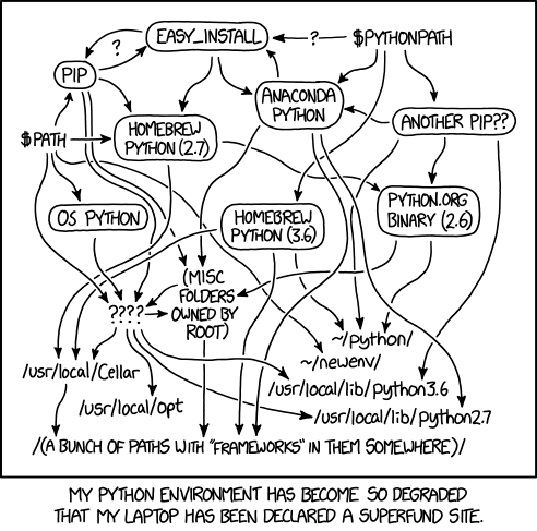
Python setup

Python relies a lot on virtual environments: each project should have its own environment that contains the Python version and the libraries used in the project.

This is to avoid conflicts between different requirements:

• project A requires polars <= 1.20.0
• project B requires polars >= 1.22.0

If we had only a system-wide installation of polars, we would constantly have to reinstall one or the other.

Having one virtual environment per project allows better project reproducibility.

Python setup

For the entire setup, I recommend using uv:

• deals with installing both Python and the libraries
• user-friendly error messages
• very fast

Basically 4 commands to remember (once uv is installed):

• uv init my-project (or uv init) creates the basic files required
• uv add to add a library to the environment
• uv sync to update the venv (e.g. after adding a dependency or to restore a project)
• uv run file.py to run a script in the project’s virtual environment

Python setup

The files uv.lock and .python-version are the only thing needed to restore a project.

You do not need to share the .venv folder with colleagues, they can just call uv sync and the .venv with the exact same packages will be created.

Python setup

For more exploratory analysis (i.e. before writing scripts meant to be run on the whole data), we can use Jupyter notebooks.

• create a new demo.ipynb file in the project folder
• run uv add ipykernel in the terminal
• in the top right corner of the editor, you should see a “Select kernel” button
• if you don’t have the “Jupyter” extension installed, the “Select kernel” button will suggest you install it (and do it)
• select the one that corresponds to our virtual environment (for me, the path ends with “brussels_teaching_january_2026/.venv”)

Python setup

Automatically formatting the code when we save the file is a nice feature (not essential for today however).

If you want this:

• in the left sidebar, go to the “Extensions” tab (the four squares icon)
• search for “Ruff” and install it
• open the “Settings” (File > Preferences > Settings)
• search for “Format on save” and tick the box
• search for “Default formatter” and select “Ruff”

and you should be good to go!

R setup

Constraints:

1. you need R >= 4.3

2. polars and tidypolars are not on CRAN, so install.packages("polars") is not enough.

Sys.setenv(NOT_CRAN = "true")
install.packages(
  c("polars", "tidypolars"),
  repos = c("https://community.r-multiverse.org", getOption("repos"))
)

renv allows you to create a virtual environment in R.